Multiphysics Learning & Networking

Theory

The root "concentration" is coined in this section to represent any process involving the evolution or/and equilibrium of the concentration field. In other words, it is used as a generic term for various mechanisms underlying mass transport of dispersed phases in the context of multiphysics. Though the mass transport of dispersed phases in a mixture, i.e., solution, colloid, and suspension, is a very basic monolithic physical process, a representative root such as concentrato has seldom been used.

A general equation for the dispersed mass transport or concentration field, including diffusion, dispersion, and advection, is formulated as equation given below. A combination of any two of them, such as diffusion and advection, is named with these two mechanisms, that is, diffusion-advection equation: \[\frac{\partial c}{\partial t} =\underbrace{\nabla \cdot \left(D_{{\rm diff}} \nabla c\right)}_{{\rm diffusion}}+\underbrace{\nabla \cdot \left(D_{{\rm disp}} \nabla c\right)}_{{\rm dispersion}}-\underbrace{v\cdot \nabla c}_{{\rm advection}}, \] where $c$ can be replaced by the other definitions of the concentration. But such a replacement requires to change the coefficients for diffusion $D_{{\rm diff}} $ and dispersion $D_{{\rm disp}} $ accordingly.

This effect is considered by multiplying the diffusion coefficient by the tortuosity ($\tau >1$). With the above considerations, Fick's first law can be modified into \[J_{{\rm diff}} =-D_{{\rm diff}}^{{\rm eff}} \nabla c, \] where $D_{{\rm diff}}^{{\rm eff}} $ is the effective diffusion coefficient. This effective diffusion coefficient is smaller than that in a continuous liquid phase due to consideration of the porosity $\phi $ and tortuosity $\tau $, \[D_{{\rm diff}}^{{\rm eff}} =\frac{\phi }{\tau } D_{{\rm diff}} , \] where tortuosity is defined as the ratio of the length of the real traveling path to the distance between the two ends of the path.

Example

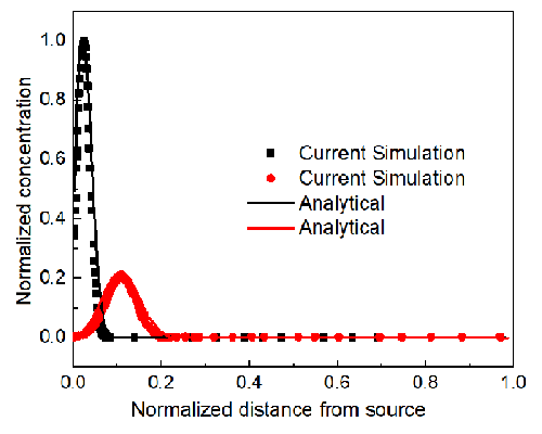
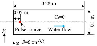
An experiment and its analytical solution for typical concentration fields were reported by Massabo et al. [2011]. As shown in the following figure, the experiment was conducted in a Perspex box, which was 0.28 m long, 0.2 m wide, and 0.01 m thick. The box was filled with transparent glass beads to simulate a porous material. There is a constant flow from the left to the right with a velocity of $2.9\times 10^{-4}$ $m/s$ along the length direction (horizontal). The combined diffusion and dispersion coefficients considering the porosity and tortuosity of the porous material are $3.322\times 10^{-7}$ $m{^2}/s$ and $2.672\times 10^{-7}$ $m{^2}/s$ along the horizontal direction and vertical direction, respectively. Dye was injected into the box at the location that is 0.05 m from the left side and 0.1 m from the top. Unfortunately, the accurate formulation of the pulse source is hard to determine based on the description in the paper. Here we can assume it is a square pulse with a magnitude of 0.1 between $t=0$ s and $t=1$ s in a circular area with a radius of 0.001 m. The initial concentration is zero across the domain. All the boundaries have no mass influx or outflux. Please simulate this experiment and compare the simulation result against the analytical solution at ${t\cdot v/L } =1/50 $ (18.96 s) and ${t\cdot v/L } =1/10 $ (t=94.8s).

For simplicity, the effective porosity is assumed to be the same as the porosity.

Result: