
Dynamic Field
Overview
Dynamics has been historically studied with respect to material types, leading to two distinct areas: elastodynamics for solids and aerodynamics (gas) and hydrodynamics (liquid) for fluids. Acoustics consists of a small part from each of the above two areas but is more focused on the vibration of the material points and the energy transfer associated with the vibration.
$\space$Elastodynamics
The wave equation of elastodynamics is simply the equilibrium equation of elastostatics with an additional inertial term: \[\sigma _{ji,j} +F_{i} =\rho \ddot{u}_{i} =\rho \partial _{tt} u_{i} . \] Substituting the linearly elastic constitutive relationship into the above equation, we can obtain the following governing equation by following a procedure similar to that was introduced in the previous chapter \[\mu u_{i,jj} +\left(\lambda +\mu \right)\mu u_{j,ji} +F_{i} =\rho \partial _{tt} u_{i} .\] Using the tensor notation, the above governing equation of elastodynamics turns into \[\mu \nabla ^{2} u+\left(\lambda +\mu \right)\nabla \left(\nabla \cdot u\right)+F=\rho \frac{\partial ^{2} u}{\partial t^{2} } . \] To obtain a better understanding of the acoustics in solids, we can separate the two major types of waves: pressure wave (P-wave, primary wave or longitudinal wave) from the shear wave (S-wave or transverse/transversal wave). For the pressure wave, there is only volumetric changes but no shearing. Mathematically, this type of physical field can be formulated as $\nabla \cdot u\ne 0$ and $\nabla \times u=0$. The physical field with such a dependent variable is called an irrotational field, a curl-free/curl-less field, or a longitudinal field. For the shear wave, there is no volumetric changes but only shearing. Mathematically, this type of field can be formulated as $\nabla \cdot u=0$ and $\nabla \times u\ne 0$. The physical field with such a dependent variable is called a solenoidal field, an incompressible field, a divergence-free field, a transverse field, or an equivoluminal field. To separate the two types of waves, we can recall the following identity from the tensor analysis \[\nabla \times \left(\nabla \times u\right)=\nabla \left(\nabla \cdot u\right)-\nabla ^{2} u. \] Then Navier's equation can be reformulated into the following equation by neglecting the body force, \[\left(\lambda +2\mu \right)\nabla \left(\nabla \cdot u\right)-\mu \nabla \times \left(\nabla \times u\right)=\rho \frac{\partial ^{2} u}{\partial t^{2} } .\] Then in the case of pressure waves, we obtain \[\left(\lambda +2\mu \right)\nabla \left(\nabla \cdot u\right)=\rho \frac{\partial ^{2} u}{\partial t^{2} } .\] The wave velocity is the square root of the ratio between the ``modulus'' and the density, i.e., $\sqrt{\frac{\lambda +2\mu }{\rho } } $. In the case of shear waves, we obtain \[-\mu \nabla \times \left(\nabla \times u\right)=\mu \nabla ^{2} u=\rho \frac{\partial ^{2} u}{\partial t^{2} } , \] where the shear wave velocity is $\sqrt{\frac{\mu }{\rho } } $.
$\space$Fluid Dynamics and Acoustics in Fluids
In fluids such as water, it is more common to derive the propagation of sound waves from the equation of continuity, i.e., conservation of mass and the equation of motion, i.e., conservation of momentum, instead of Navier's equation as for solids. $\frac{\partial p}{\partial t} +k\nabla \cdot v=0$ (mass balance) $\rho _{0} \frac{\partial v}{\partial t} +\nabla p=0$ (momentum balance) where $p$ is the acoustic pressure, which can be viewed as the deviation from the hydraulic pressure in fluid dynamics due to the existence of the wave, and $v$ is theflow velocity excluding the background velocity associated with the background fluid dynamics.
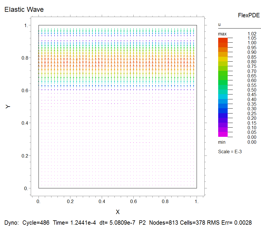
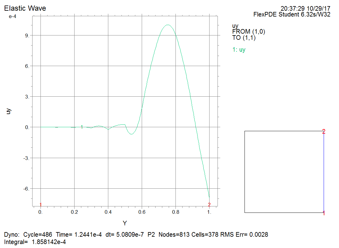
$\space$Example
This problem is modified from the practice problem in the mechanical field chapter. A square element with a side length of 1 m is composed of a material with a Young's modulus of 10 GPa, a Poisson's ration of 0.2, and a density of 1000. An electric wave is generated by repeatedly compressing and stretching the upper boundary of the element at a given frequency. Please simulate the wave inside the element to tell what you observe at a frequency of 500 Hz and 5000 Hz and explain the reason for the difference.