

Poroelasticity
Introduction
Poroelasticity is traditionally used to describe the coupling between the solid and the interpenetrating fluid in their mixture, in which the solid is believed to be saturated by the fluid. In other words, it is an area of studying the movement/flow of material points in both the liquid phase and the solid skeleton. This is distinct from both the groundwater movement and mechanical/dynamic responses of the skeleton. For example, the hydraulic field based on Darcy's law does not take into account the fact that the solid skeleton can be altered.
There are two major parts for poroelasticity: static (or quasi-static) and dynamic theories. The static poroelasticity accounts for a process in which water movement and solid skeleton deformation occur simultaneously and affect each other. Therefore, it can be termed as hydromechanics. This static poroelasticity theory is a generalization of the consolidation theory in soil mechanics. As a result, poroelasticity is frequently used interchangeably with the consolidation theory or to refer to the static poroelasticity in a narrow sense. The dynamic poroelasticity is developed for the wave propagation in both the liquid and solid phases of saturated porous materials.
$\space$Static Poroelasticity
The establishment of the constitutive relationships for saturated porous materials needs to consider both the solid and fluid. It is not difficult to imagine that these two phases will interact with each other in the stress-strain relationship. Since the fluid stress/strain only has normal components, the couplings between the solid and fluid only occur via these normal terms. As a result, we usually identify the couplings between normal or bulk/volume stress/strain first and then add in the shear terms in the formulation. The following constitutive relationship can be obtained:
\[\varepsilon _{{\rm v}} =\frac{\sigma }{K} +\frac{p}{H} , \] \[\zeta =\frac{\sigma }{H} +\frac{p}{R} , \]where $K$ is the bulk modulus, $H$ is the poroelastic expansion coefficient, and $R$ is the reciprocal of the unconstrained storage coefficient.
The above constitutive relationships are sometimes written in the following form:
\[\sigma =K\varepsilon _{{\rm v}} -\alpha p, \] \[\zeta =\alpha \varepsilon _{{\rm v}} +\frac{1}{M} p, \]where $\alpha =\frac{K}{H} $ is the Biot-Willis coefficient introduced above and $\frac{1}{M} =\frac{1}{R} -\frac{K}{H^{2} } $ is the constrained specific storage coefficient. It is seen that, in either form of the constitutive relationship, only three independent mechanical properties are needed. In order to use the above relationships to derive the governing equation, the shear stress/strain needs to be included. The complete constitutive relationship for the static poroelasticity is
\[\sigma _{ij} =\lambda \varepsilon _{kk} \delta _{ij} +2G\varepsilon _{ij} -\alpha p\delta _{ij} =\lambda \cdot trace\left(\varepsilon \right)+2G\varepsilon -\alpha pI, \] \[\zeta =\alpha u_{i,i} +\frac{1}{M} p=\alpha \nabla \cdot u+\frac{1}{M} p. \]Substituting the constitutive equations into the Navier's equation for the momentum equilibrium of the solid and continuity equation of the pore fluid, we obtain the final governing equations
\[\left(\lambda +\mu \right)\nabla \left(\nabla \cdot u\right)+\mu \nabla ^{2} u+f=\alpha \nabla p, \] \[\frac{1}{M} \frac{\partial p}{\partial t} +\nabla \cdot \left[-\frac{k}{\eta } \nabla \left(p+z\right)\right]=-\alpha \frac{\partial }{\partial t} \left(\nabla \cdot u\right),\] where $k$ is the permeability.In poroelasticity, we may also see some other material properties, which can be formulated using $K$, $H$, $R$ , and so on. These include the undrained modulus,
\[K_{u} =\frac{\delta \sigma }{\delta \varepsilon _{v} } \left|{}_{\zeta =0} \right. =\frac{1}{\frac{1}{K} -\frac{R}{H^{2} } } ,\]undrained Poisson's ratio,
\[\nu _{u} =\frac{3\nu +\alpha B\left(1-2\nu \right)}{3-\alpha B\left(1-2\nu \right)} , \]and first Skempton's coefficient,
\[ B=\frac{\partial p}{\partial \sigma} |_{\zeta=0} = -\frac{R}{H} = \alpha M/K_{u} \]Further micromechanical relationships are sometimes needed to relate the material properties of the porous material to its phases [Merxhani, 2016]:
\[\alpha =1-\frac{K}{K_{{\rm s}} }\space [Biot \space and \space Willis, 1957] \] \[\frac{1}{M} =\frac{1}{R} -\frac{\alpha }{H} =\left(1-\frac{K}{K_{{\rm s}} } -\phi \right)\frac{1}{K_{{\rm s}} } +\phi \frac{1}{K_{{\rm f}} } \space [Verruijt, 1969] \]This will lead to
\[\frac{1}{H} =\frac{1}{K} -\frac{1}{K_{{\rm s}} } ,\] \[\frac{1}{R} =\frac{1}{K} +\phi \left(\frac{1}{K_{{\rm f}} } -\frac{1}{K_{{\rm s}} } \right)-\frac{1}{K_{{\rm s}} } ,\]where $K_{{\rm s}} $ and $K_{{\rm f}} $ are the bulk moduli of the solid and fluid phases, respectively. In many documents, compressibilities (reciprocals of bulk moduli) instead of bulk moduli are used in the above equations.
$\space$Dynamic Poroelasticity
In static poroelasticity, the inertial and associated kinetic energy were not considered. However, when the speed of the movement of the phases in the porous material is appreciable, e.g., when there is vibration or stress waves, the theory in the previous section cannot well describe the behavior of the porous materials. To include these dynamic effects, constitutive relationships are slightly modified from those adopted in the previous section:
\[\sigma _{s} =A\varepsilon _{{\rm v}} \delta +Qe+2G\varepsilon \] \[p=Q\varepsilon _{{\rm v}} \delta +Re\] \[E_{p} =\frac{1}{2} \left(\sigma _{s} \cdot \varepsilon +p\cdot e\right), \]where $G$, $A$, $Q$, and $R$ are another four parameters quantifying the elastic properties of the porous material. They are not conventional moduli but can be obtained using the moduli of the phases and the bulk mixture.
To derive the governing equation, it is better to recall the Lagrangian equation. The Lagrangian mechanics is just another description of the classic mechanics which works better for complicated systems involving a lot of constraints. The Lagrange equation is
\[\frac{d}{dt} \frac{\partial }{\partial \dot{x}} \left(E_{{\rm k}} -E_{{\rm d}} \right)-\frac{\partial }{\partial x} \left(E_{{\rm k}} -E_{{\rm d}} \right)=F, \]where $x$ is the generalized coordinate(s), $E_{{\rm k}} $ is the kinetic energy, $E_{{\rm d}} $ is the energy dissipation, and $F$ is the total force. The kinetic energy is
\[E_{{\rm k}} =\frac{1}{2} \left(\rho _{11} \dot{u}\cdot \dot{u}+\rho _{11} \dot{U}\cdot \dot{U}+2\rho _{12} \dot{u}\cdot \dot{U}\right), \]where $\rho _{11} $, $\rho _{22} $, and $\rho _{12} $ are the effective density of the solid, liquid, and coupling between the solid and the liquid respectively. These density terms can be related to the densities of the solid and liquid via the following equations [Biot, 1956a, b]:
\[\rho _{11} =\left(1-\phi \right)\rho _{{\rm s}} -\rho _{12} ,\] \[\rho _{22} =\phi \rho _{{\rm f}} -\rho _{12} , \] \[\rho _{12} =-\left(\tau -1\right)\phi \rho _{{\rm f}} . \]The energy dissipation function can be expressed in terms of the velocities of the solid and fluid,
\[E_{d} =\frac{1}{2} b_{0} \left(\dot{u}-\dot{U}\right)\cdot \left(\dot{u}-\dot{U}\right), \]where the coefficient $b_{0} $ can be related to the permeability, dynamic viscosity, and porosity via the following equation:
\[b_{0} =\frac{\eta \phi ^{2} }{k} .\]Substituting the above constitutive relationships and energy functions into the Lagrange equation, we can obtain the following governing equations:
\[\rho _{11} \ddot{u}+\rho _{12} \ddot{U}+b_{0} \left(\dot{u}-\dot{U}\right)=\left(A+G\right)\nabla \left(\nabla \cdot u\right)+G\nabla ^{2} u+Q\nabla \left(\nabla \cdot U\right)+F_{{\rm s}} -Q\nabla \theta _{{\rm s}} \] \[\rho _{12} \ddot{u}+\rho _{22} \ddot{U}-b_{0} \left(\dot{u}-\dot{U}\right)=Q\nabla \left(\nabla \cdot u\right)+R\nabla ^{2} U+F_{{\rm f}} -R\nabla \theta _{{\rm f}} . \] $\space$Example
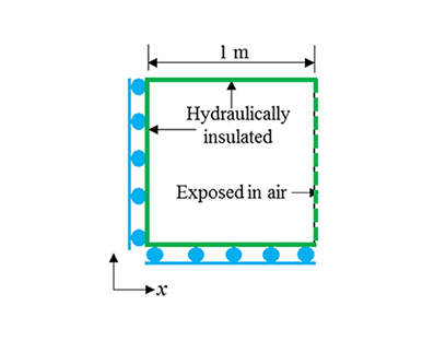
In linear poroelasticity, Mandel's problem [Mandel, 1955; Abousleiman et al., 1996] is usually used to validate linear poroelastic models. Mandel [1955] presented an analytical solution to predict the coupled hydromechanical response of porous materials under a set of prescribed boundary conditions [Ferronato et al., 2010]. In the Mandel's problem, a 2D rectangular object (plane strain) is subjected to a vertical distributed load of $p_{0} $ while the two side boundaries are free to move. The top and bottom boundaries are hydraulically insulated while the side boundaries are exposed in air (zero pore water pressure). Due to the symmetry in the geometry and loading, we can only analyze one fourth of the object. Accordingly, a 2D domain that has dimensions of 1 m by 1 m (a$\times $b) is adopted here. Let us consider the upper right fourth of the 2D object. Therefore, the left and bottom boundaries will be symmetric. That is, there is no normal displacement and no shear stresses for the mechanical field while no flux is allowed through the boundaries (hydraulic insulation).
The analytical solution for such a problem is
\[p=2p_{0} \sum _{n=1}^{\infty }\left[\frac{\sin \alpha _{n} }{\alpha _{n} -\sin \alpha _{n} \cos \alpha _{n} } \left(\cos \frac{\alpha _{n} x}{a} -\cos \alpha _{n} \right)\exp \left(\frac{-\alpha _{n}^{2} ct}{a^{2} } \right)\right] , \]where $\alpha _{n} $ is the $n$th positive solution to the following equation:
\[\tan \alpha =\frac{\lambda +2\mu }{\mu } \alpha , \]and $c$ is the consolidation coefficient and can be calculated using poroelastic and other material properties as
\[c=\frac{\kappa }{\rho _{w} {\rm g}\left(\frac{1}{M} +\frac{\alpha ^{2} }{\lambda +2\mu } \right)} , \]in which $\kappa $ is the hydraulic conductivity.
In our example, the two Lam'e constants are both 40 MPa, the Poisson's ratio is 0.3, the Biot-Willis coefficient is 1.0, the porosity is 0.375, the hydraulic conductivity is $1\times 10^{-5} $ the compressibilities of the pore water and solid grain are $4.4 \times 10^{-10} $ and $2.8\times 10^{-10} $ respectively. Please calculate the pore water distributions at 0.05 s, 0.5 s, 5 s, and 10 s, and compare them against the analytical solution
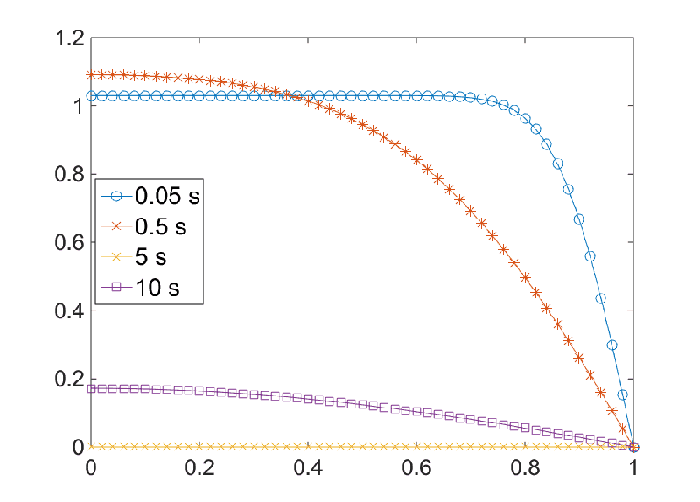
The analytical solution is shown in the above figure, which clearly shows the peculiar non-monotonic pressure behavior, i.e. the so-called Mandel-Cryer effect, in which $p$ rises above the initial $p_{0} $ at small time values. This non-monotonic pressure change occurs because the slab contraction at the drained faces induces an additional build-up of pressure in the interior.