
Magnetostatic Field
Theory
The magnetic field can be formulated using the magnetic vector potential. Different from the electric field, which is irrotational, the magnetic field is equivoluminal (sourceless or solenoidal). That is, the magnetic flux density satisfies a zero-divergence condition, therefore, $B$ can be represented as the curl of another vector such that \[B=\nabla \times A, \] where $A$ is the magnetic vector potential. Substituting the above equation into Gauss's law for the magnetic field, we obtain \[\nabla \cdot \left(\nabla \times A\right)=0. \] As can be seen, this equation is automatically satisfied, which confirms the effectiveness of the use of the magnetic vector potential. The above equation needs to be substituted into the Ampère's law to yield the governing equation in terms of the vector potential. \[\nabla \times \left(\frac{\nabla \times A}{\mu _{0} } +M\right)=J.\] If the linear relationship between $B$ and $H$ can be assumed, we can obtain \[\nabla \times \left(\frac{\nabla \times A}{\mu _{0} \mu _{r} } \right)=J.\] As we know, except in metals, electric currents can be ignored in materials. Then the above equation is reduced into \[\nabla \times \left(\frac{\nabla \times A}{\mu _{0} \mu _{r} } \right)=0.\] The above standard governing equation can be further simplified by introducing extra constraints on $A$. First, let us use the absolute permeability, \[\nabla \times \left(\frac{1}{\mu } \nabla \times A\right)=0.\] Then we apply Lagrange's formula to transform the above equation into \[\nabla \times \left(\frac{1}{\mu } \nabla \times A\right)=\nabla \left(\frac{1}{\mu } \nabla \cdot A\right)-\nabla \cdot \left(\frac{1}{\mu } \nabla A\right)=0. \] As $A$ is a quantity that we construct, we can impose any further constraints when constructing $A$ as long as the above conditions are not violated. For example, we can set $\nabla \cdot A=0$, which is called the Coulomb gauge condition. Then we have \[\nabla \cdot \left(\frac{1}{\mu } \nabla A\right)=0. \] For permanent magnets, permanent magnetization exists while electric currents are absent, so we have \[\nabla \times \left(\frac{\nabla \times A}{\mu _{0} } -M\right)=0, \] or with the Coulomb gauge condition as \[\nabla \cdot \left(\frac{1}{\mu _{} } \nabla A\right)-\nabla \times M=0.\] The introduction of this vector potential does not appear as useful and common as the electric potential in the electric field. However, the vector potential will help a lot when we move from magnetostatics to electromagnetics.
Corresponding to the electric field, the magnetic potential energy of a continuum can be formulated as \[U=\frac{1}{2} \int _{V}H\cdot BdV =\frac{\mu }{2} \int _{V}H\cdot HdV =\frac{1}{2\mu } \int _{V}B\cdot BdV .\] The electric potential energy density of the magnetic field can be formulated using either $\mu H^{2}/2 $ or $B^{2} /(2\mu) $, in which $H$ and $B$ are the magnitudes of the $H$ and $B$ field, respectively.
$\space$Example
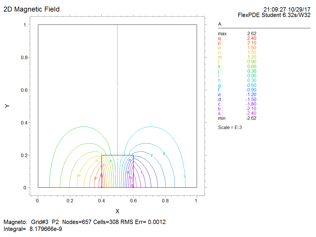
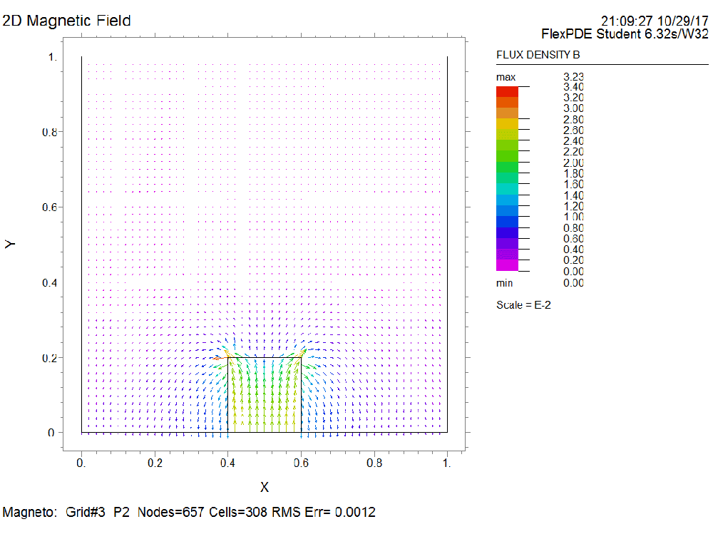
Please simulate the magnetic field generated by a bar magnet that is 0.4 m long and 0.2 m wide (2D) in vacuum. The magnet has magnetic polarization along the length direction whose magnitude is 10000 A/m. The relative permeability of the magnet material is 5000.