Multiphysics Learning & Networking

Theory

The governing equation for heat transfer can be easily obtained based on the conservation equation, \[\frac{\partial e}{\partial t} +\nabla \cdot \left(ev\right)+\nabla \cdot J_{{\rm T}} =q_{{\rm T}} ,\] where the subscript, T, denotes the conservation of energy, which is the extended definition of thermal fields. The conservation of quantities and the corresponding physical fields are used interchangeably throughout this website.

In order to get a heat transfer equation that we are more familiar with, let us start from the formation of the energy density term, \[e=\underbrace{\left(\int _{T_{0} }^{T}\rho C_{{\rm v}} T +U_{0} \right)}_{{\rm Internal\; Energy}}+\underbrace{\left(\frac{1}{2} \rho v\cdot v\right)}_{{\rm Kinetic\; Engergy}}+\underbrace{\left(\rho {\rm g}z\right)}_{{\rm Potential\; Energy}}, \] where $C_{{\rm v}} $ is the gravimetric heat capacity at a constant volume and $U_{0} $ is the internal energy per unit volume at the reference temperature $T_{0} $.

The internal energy is part of the accumulation term in addition to the kinetic energy and potential energy. But in general, the internal energy is dominant over the other energy types. As a result, the energy density is frequently represented by only the internal energy density as equation below, in which the pressure term vanishes for solids, \[e=\int _{T_{0} }^{T}\rho C_{{\rm v}} T +U_{0} =\int _{T_{0} }^{T}\rho C_{{\rm p}} T -\int pdV +U_{0} ,\] where $C_{{\rm p}} $ is the heat capacity at a constant pressure.

Next, the flux term is linked to the temperature by Fourier's law of heat conduction as \[J_{{\rm T}} =-\lambda \nabla T,\] where $\lambda $ is the thermal conductivity. Substituting the above equations for energy density and heat flux into the energy balance equation, we can obtain the heat equation including advection and source terms as \[\frac{\partial \left(\rho C_{{\rm v}} T\right)}{\partial t} +\nabla \cdot \left(\rho C_{{\rm v}} Tv\right)-\nabla \cdot \left(\lambda \nabla T\right)=q_{{\rm T}} .\] As can be seen, this equation is a comprehensive version of the Fourier's equation for heat transfer. The above deduction shows how to obtain the equation from the basic heat conservation law.

The Dirichlet boundary condition is used to handle the condition when the temperature on a boundary is known. For the purpose, a known value of temperature T${}_{env}$ is assigned to the vertex or the edge of the computational domain. This is common in chemical reactions when we have a water bath with a constant temperature in contact with the boundary. The T${}_{env}$ value at the edge can be specified as a linear function of coordinates. The function parameters can vary from one edge to another but have to be adjusted to avoid discontinuities at edges' junction points. This boundary condition sometimes is called the boundary condition of the first kind.

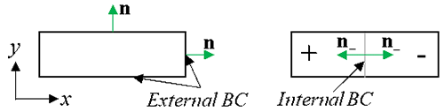
The Neumann boundary condition is used to consider the condition when the heat flux across a boundary is prescribed.This type of boundary condition can be applied to external boundaries or internal boundaries between regions: \[-n\cdot J=-F_{n} \space\space\space\space at\space external \space boundaries, \] \[-n_{+} \cdot J_{+} -n_{-} \cdot J_{-} =F_{n} \space\space\space\space at\space internal\space boundaries.\] For external boundaries, F${}_{n}$ is the outward normal component of heat flux. For the internal boundary, "+" and "-" superscripts denote quantities to the left and to the right side of the boundary by assuming the axis is pointing to the right. The left region is "+" because it has a boundary outward normal vector pointing in the positive direction. On the internal boundary, $F_{n} $ is the generated power per unit area or equivalently the surface source.

The convection boundary condition describes convective heat transfer. The convective heat transfer can be described using Newton's law of cooling, in which the heat flux is proportional to the difference between the temperature of the material adjacent to the boundary and the ambient temperature. This type of boundary condition including Newton's law of cooling is defined as \[F_{n} =h\left(T-T_{{\rm env}} \right),\] where $h$ is the coefficient of convective heat transfer and $T_{{\rm env}} $ is the temperature of contacting fluid medium. Parameters $h$ and $T_{{\rm env}} $ may differ from part to part of the boundary.

The Neumann boundary condition can also be extended to consider radiative heat transfer across boundaries: \[F_{n} =\beta k_{{\rm SB}} \left(T^{4} -T_{{\rm env}}^{4} \right),\] where $k_{{\rm SB}} $ is a Stephan-Boltzmann constant (5.67032·10${}^{-8\ }$W/m${}^{2}$/K${}^{4}$), and $\beta $ is an emissivity coefficient. Parameters $\beta$ and $T_{0} $ may differ from part to part of the boundary.

Example

In rectangular Cartesian coordinates shown in the figure below, the 2D sourceless heat equation can be simplified into the following form when the density, heat capacity, and thermal conductivity are constants: \[\frac{\partial w}{\partial t} =a(\frac{\partial ^{2} w}{\partial x^{2} } +\frac{\partial ^{2} w}{\partial y^{2} } ), \] where $w$ is the dependent variable, which is the temperature in this case; and $a$ is the thermal diffusivity. The material filling the domain is water.

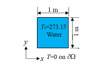
1. The problem to be solved corresponds to a 2D square region (1 m by 1 m). The initial temperature is 273.15 K throughout the interior of the region. The temperature on all the boundaries is fixed as 0 K. The question is how the temperature in the domain changes in the first hour. Please describe the problem using mathematical terms.

2. Please conduct simulations using the PDE toolbox in Matlab. Explain the process step by step (print your screen and add some text to explain what you do).

3. Compare the numerical results with the analytical solution as follows: \[w=\frac{16w_{0} }{{\rm \pi }^{2} } \left\{\sum _{n=0}^{\infty }\frac{1}{2n+1} \sin \left[\frac{\left(2n+1\right){\rm \pi }x}{l_{1} } \right]\exp \left[-\frac{{\rm \pi }^{2} \left(2n+1\right)^{2} at}{l_{1} {}^{2} } \right] \right\}\] \[\times \left\{\sum _{n=0}^{\infty }\frac{1}{2m+1} \sin \left[\frac{\left(2m+1\right){\rm \pi }y}{l_{2} } \right]\exp \left[-\frac{{\rm \pi }^{2} \left(2m+1\right)^{2} at}{l_{2} {}^{2} } \right] \right\}.\]

To save your time, a MATLAB program has been developed for implementing the analytical solution. But you still need to extract values from both numerical and analytical solutions so that you can do a quantitative evaluation. For example, you can try to compare the temperature distributions along y=0 at t=3600. For the numerical solution, you will need to export mesh and solution from the toolbox GUI first. Then can you use a MATLAB command tri2grid to get the solution on a straight line, i.e., tri2grid(p,e,u(:,3600),-0.5:0.01:0.5,0). As for the distributions in the analytical solution, you can extract the values using a couple of commands as long as you know the structure of the solution (spend a few minutes to understand the code in the appendix). Refine the mesh in the PDE toolbox and run the simulation again. Please show whether the accuracy of the solution is improved.