Multiphysics Learning & Networking

Introduction

One essential idea behind numerical simulation is discretization. For the purpose, we need to transform a continuous mathematical equation (s) into an algebraic equation. Accordingly, the computational domain will be discretized into a mesh or a grid which consists of multiple subdomains called cells or elements. The size of the matrices in the algebraic equation is determined by the mesh size, the dimensions of the computational domain, and the number of unknowns. Therefore, the discretization of the equations and that of the domains are correlated. Different ways or schemes can be used to approximate the same derivative, leading to different levels of accuracy. In addition, discretization of spatial derivatives and temporal derivatives are also different due to the difference between the spatial and temporal dimensions. For a spatial dimension, we always know the conditions on the "start" end and need to march toward the "final" end; while for spatial dimensions, boundary conditions could be given on any ends (boundary segments) or even both. This leads to the different terms and ways used for these two types of discretization.

Spatial Discretization

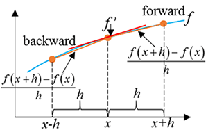
The idea of the finite difference method is to use the above quotient, $D\left(u\right)$, to approach the gradient (derivative) at the point $x$, point $x+h$ or any point between them. The geometric analogy of this approximation is to use a secant line to approximate a tangent line. For the first-order derivative, the most common schemes are forward, backward, and central difference schemes. A forward scheme has an expression of the form \[f'\left(x\right)=\frac{f\left(x+h\right)-f\left(x\right)}{h}\] It is called "forward" because we use the function value at a point in front of (along the direction of the corresponding axis) the point at which the derivative is calculated. Likewise, a backward scheme uses the function values at $x$ and $x-h$ instead: \[f'\left(x\right)=\frac{f\left(x\right)-f\left(x-h\right)}{h}\] We can also approximate the derivative using the function values at points on the two sides of the point of derivative as \[f'\left(x\right)=\frac {{{f\left(x+h/2\right)}-{f\left(x-h/2\right)}}}{h}\] A second-order derivative can be approximated using first order derivatives as we can view the second-order derivative as a derivative of first-order derivatives. For example, in order to obtain the second-order derivative at the point $x$, we can use the derivatives at the points $\left(x-h/2\right)$ and $\left(x+h/2\right)$: \[f''\left(x\right)=\frac{f'\left(x+h/2\right)-f'\left(x-h/2\right)}{h}\] The above approximation uses the central difference. We can also use central differences for the first derivative in the above equation, leading to \[\begin{array}{l} {f''\left(x\right)=\frac{\frac{f\left(x+h\right)-f\left(x\right)}{h} -\frac{f\left(x\right)-f\left(x-h\right)}{h} }{h} } \\ {{\rm \; \; \; \; \; \; \; \; \; \; }=\frac{f\left(x-h\right)-2f\left(x\right)+f\left(x+h\right)}{h} } \end{array}\]

Temporal Finite Difference and Schemes

Let us first reformulate the general transient partial differential equation in the following way: \[u_{t} =f\left(u\right),\] where $f\left(u\right)$ in the equation contains all the terms except the temporal derivative term. First, for the temporal difference, let us use the following most common form as our purpose is to calculate the function value at the next time step $n+1$ based on the known function value at the current time step $n$: \[\frac{u^{n+1} -u^{n} }{k} =f\left(u\right),\] where $k$ is the time step. An Euler forward scheme is used for the temporal derivative. The word "Euler" differentiates the temporal schemes from the spatial schemes. The choice of $u$, i.e. $u$ from which time step, determines the type of the temporal scheme. If all the unknown values are from the current step, then the scheme is explicit, \[\frac{u^{n+1} -u^{n} }{k} =f\left(u^{n} \right). \] The following solution can be readily obtained for this scheme: \[u^{n+1} =u^{n} +k\cdot f\left(u^{n} \right).\] The above two types of schemes can also be mixed to construct other schemes: \[\frac{u^{n+1} -u^{n} }{k} =\left(1-\theta \right)f\left(u^{n} \right)+\theta f\left(u^{n+1} \right),\] where $\theta $ is the ratio. $\theta $ values of 0 and 1 lead to explicit and fully implicit schemes, respectively; while those values between 0 and 1 produce partially implicit ones. Another common implicit scheme, the Newton-Nicolson scheme will be obtained when $\theta $ equals 0.5. Partially implicit schemes are also unconditionally stable.

Example

Point 1: $\frac{u_{1}^{n+1} -u_{1}^{n} }{k} =\frac{u_{0}^{n} -2u_{1}^{n} +u_{2}^{n} }{h^{2} } $

Point 2: $\frac{u_{2}^{n+1} -u_{2}^{n} }{k} =\frac{u_{1}^{n} -2u_{2}^{n} +u_{3}^{n} }{h^{2} } $

$\dots $

Point $i$ : $\frac{u_{i}^{n+1} -u_{i}^{n} }{k} =\frac{u_{i-1}^{n} -2u_{i}^{n} +u_{i+1}^{n} }{h^{2} } $

$\dots $

Point $I$ : $\frac{u_{I}^{n+1} -u_{I}^{n} }{k} =\frac{u_{I-1}^{n} -2u_{I}^{n} +u_{I+1}^{n} }{h^{2} } $

If we incorporate the above boundary conditions, we will get

Point 1: $\frac{u_{1}^{n+1} -u_{1}^{n} }{k} =\frac{a-2u_{1}^{n} +u_{2}^{n} }{h^{2} } $

Point 2: $\frac{u_{2}^{n+1} -u_{2}^{n} }{k} =\frac{u_{1}^{n} -2u_{2}^{n} +u_{3}^{n} }{h^{2} } $

$ \dots $

Point $i$ : $\frac{u_{i}^{n+1} -u_{i}^{n} }{k} =\frac{u_{i-1}^{n} -2u_{i}^{n} +u_{i+1}^{n} }{h^{2} } $

$\dots $

Point $I$ : $\frac{u_{I}^{n+1} -u_{I}^{n} }{k} =\frac{u_{I-1}^{n} -u_{I}^{n} +\beta h}{h^{2} } $