
Electrostatic Field
Theory
The definition of the electric potential, combined with the differential form of Gauss's law, provides the following governing equation for the electric field: \[\nabla ^{2} \psi =-\frac{\rho }{\varepsilon _{0} } . \] This equation is in the form of Poisson's equation. In the absence of electric charges, the equation degenerates into Laplace's equation: \[\nabla ^{2} \psi =0. \] This PDE can be solved with appropriate boundary conditions. A Dirichlet boundary condition for an electric field just gives out the electric potential on the boundary. For example, when the boundary is far enough from charges, we can assume the boundary is infinitely far and thus has an electric potential of zero. By contrast, a Neumann boundary condition places a constraint on the gradient of the electric potential, i.e., electric field. For example, for any conductor in an electric field, the direction of the electric field needs to be parallel to the outward normal of the surface. Therefore, the component of the electric field parallel to the surface (or perpendicular to the outward normal vector) will be zero. The electrostatic energy then has the following formulation \[U=\frac{\varepsilon }{2} \int _{V}E\cdot EdV . \] Based on the above introduction, the electric potential energy density of the electric field can be formulated using either ${\rho \psi}/2$ or ${\varepsilon} E^{2}/2$.
$\space$Example
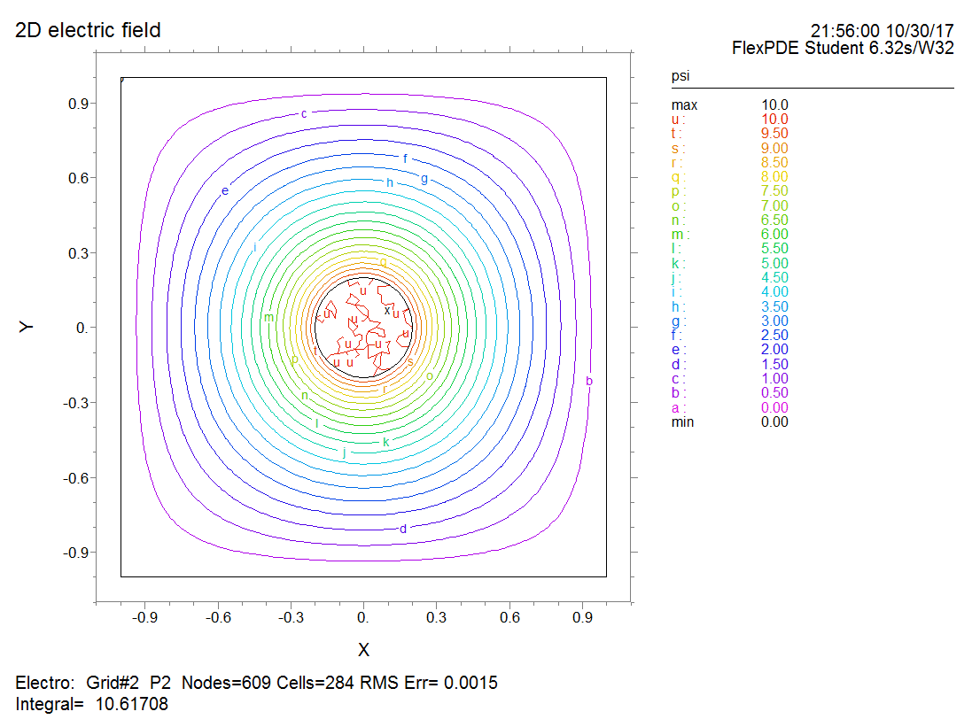
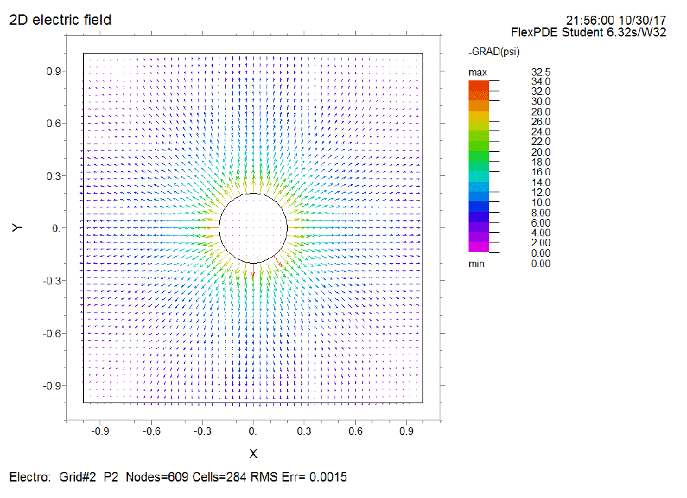
Please simulate the electric field generated by a metal cylinder whose electric potential is 10 V. The metal cylinder has a radius of 0.2 m and the length is much larger than the radius.