Multiphysics Learning & Networking

Introduction

Electromagnetics, or electromagnetism, deals with physical processes in which both the electric field and magnetic field are involved. Unlike an individual electrical field and an individual magnetic field, which exists independently as electrostatics and magnetostatics, respectively, the electrical field and magnetic field in electromagnetics are varying (dynamic) and each can cause the other, leading to a fully coupled multiphysical process.

For the electromagnetic field of interest here, Maxwell's equations are the primary mathematical descriptions. Maxwell's equations in the tensor form include four partial differential equations and a few auxiliary constitutive relationships between several terms in these partial differential equations. Maxwell's equations describe how electric and magnetic fields are generated and altered by each other and by charges and currents.

Maxwell's Equations

The equations in SI units can be formulated as follows.

where $D$ is the electric displacement (field), $\rho _{{\rm e}}^{{\rm f}} $ is the free charge density, $E$ is the electric field, $B$ is the magnetic field, $H$ is the magnetizing field or the auxiliary magnetic field, and $J_{{\rm e}}^{{\rm f}} $ is the free current density.

The above four equations contain seven unknowns. Therefore, three more constitutive relationships are needed to close the mathematical description:

where $\varepsilon $ is the absolute permittivity, $\mu $ is the permeability, $\sigma _{{\rm e}} $ is the electrical conductivity. The last constitutive equation is Ohm's law.

Boundary Conditions

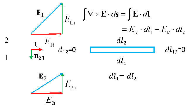
The boundary conditions can be derived from the governing equations by ensuring the validity of the equations on the boundary. The derivation is more complicated than other physical fields due to 1) the number of equations, 2) the vector form of the dependent variables and 3) the involvement of the cross product operators. The following figure illustrates a simple derivation for Faraday's equation. Let us consider a small slender rectangular area bounded by the blue lines along the boundary between the two regions. Application of the Stokes theorem to Faraday's equation will lead to $E_{1t} \cdot dl_{1} -E_{1t} \cdot dl_{2} =0$ if the area is infinitely slender, i.e., $dl_{12} \approx 0$. Because $dl_{1} =dl_{2} $, we obtain $E_{1t} =E_{1t} $ (or $E_{2}^{\parallel } -E_{1}^{\parallel } =0$), which is equivalent to $n_{12} \times \left(E_{2} -E_{1} \right)=0$. The other boundary conditions can be derived in similar ways.

Depending on the electric and magnetic properties, the electromagnetic fields can be discontinuous or continuous on each side of the common boundary (interface) between two different materials. In summary, on an interface between two materials, the field must satisfy the following conditions:

where $n_{12} $ the unit normal vector pointing from Region 1 to Region 2; and $u_{}^{\parallel } $ and $u_{}^{\bot } $ are the tangential and normal components respectively.

The above four equations indicate that 1) the electric field's tangential components are continuous across the interface, 2) the electric flux's normal component is discontinuous across the interface between materials and the difference is the charge density, 3) the tangential components of the magnetic field strength are discontinuous across the interface and the "jump" equals an electric current flux, and 4) the magnetic flux density's normal component is continuous across the interface [Fisk, 2008]. $\rho _{{\rm e}} $ and $J_{{\rm e}}^{{\rm f}} $ vanish under the conditions of no electric charge and no electric current, respectively.

For external boundaries, we only consider the region inside the boundary. Then the above four equations reduce into

Electromagnetic Waves

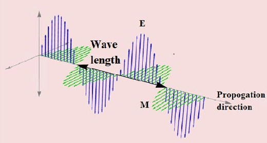
The four Maxwell's equations can be consolidated into two wave equations in special cases. Such a consolidation can be used to unify the theories of electromagnetism and optics. The 3D diagram in the following figure shows a plane linearly polarized wave propagating from left to right.

The special conditions that are required for the reformulation of the original Maxwell's equations into wave equations are 1) no charges ($\rho$= 0) and 2) no currents ($J_{{\rm e}}^{{\rm f}} $=0), such as the condition in vacuum. In such cases, Maxwell's equations reduce to

Taking the curl($\nabla \times $)of the curl operation on the last two equations, and using the curl of the curl identity, i.e.,$\nabla \times \left(\nabla \times u\right)=\nabla \left(\nabla \cdot u\right)-\nabla ^{2} u$, we obtain the wave equations: \[\frac{\partial ^{2} D}{\partial t^{2} } =\frac{1}{\varepsilon _{0} \mu _{0} } \nabla ^{2} D\] \[\frac{\partial ^{2} B}{\partial t^{2} } =\frac{1}{\varepsilon _{0} \mu _{0} } \nabla ^{2} B,\] where $c=\sqrt{\frac{1}{\varepsilon _{0} \mu _{0} } } =2.9979\times 10^{8} $ m/s is the speed of light in free space. In materials with relative permittivity $\varepsilon _{{\rm r}} $and relative permeability $\mu _{{\rm r}} $, the phase velocity of light becomes \[c=\sqrt{\frac{1}{\varepsilon _{0} \varepsilon _{{\rm r}} \mu _{0} \mu _{{\rm r}} } } , \] which is usually less than c in vacuum.

Example

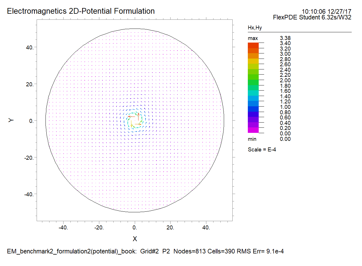
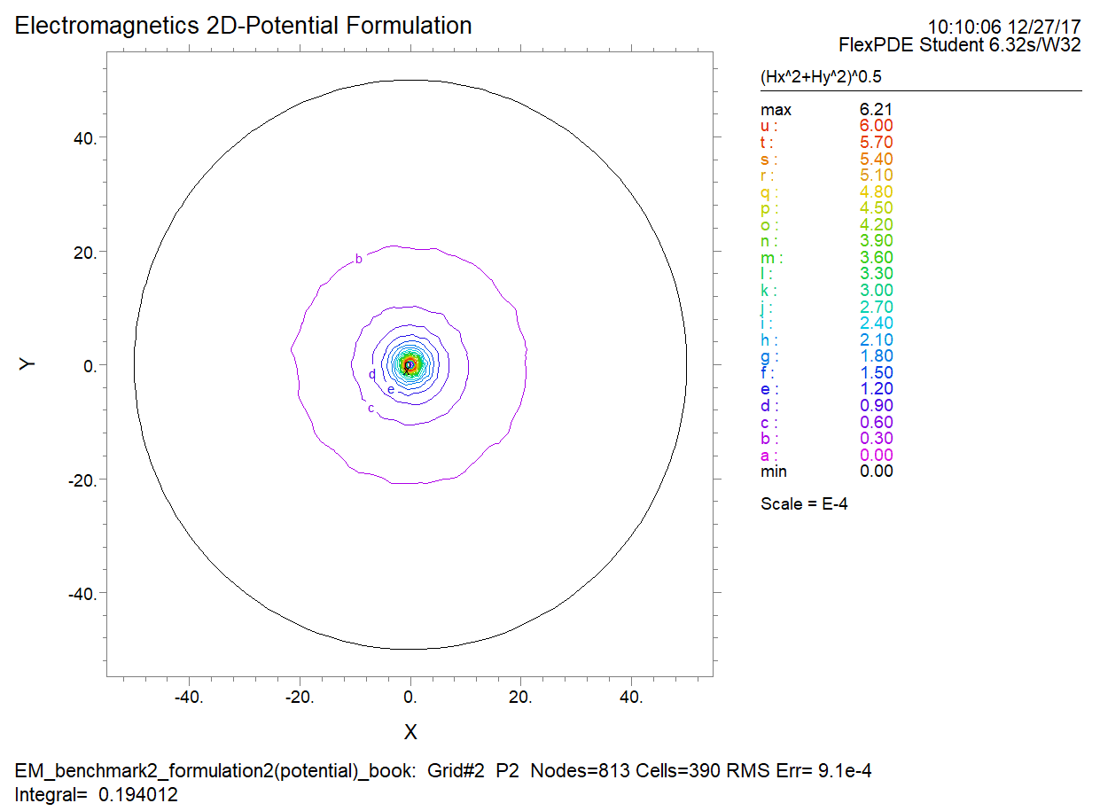
As shown in the following figure, in this benchmark problem, we consider a wire, which can be viewed as a perfect conductor, with an infinite length and a constant current of 0.01 A/m${}^{2}$ in it.

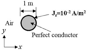
The material surrounding this wire is air. The wire is aligned in the z-direction and has a diameter of 1 m. Please simulate the $H$ field using 2D numerical simulation. Please simplify the governing equation(s) from 3D to 2D first. This is a good practice to get familiar with Maxwell's equations. Please compare the distributions of the potential along the radial direction obtained by the potential method and field vector method.