
Mechanical Field
Theory
The governing equation for the mechanical field can be obtained based on the balance law: Cauchy's equations of motion. According to the principle of conservation of linear momentum, if the continuum body is at mechanical equilibrium, it can be demonstrated that the components of the Cauchy stress tensor at every material point in the body satisfy the equilibrium equations. Let us consider a continuum body occupying a volume $V$, having a surface area $S$, with defined traction or surface forces $T_{i}^{(n)} $ per unit area acting on every point of the body surface, and body forces $F_{i} $ per unit of volume on every point within the volume $V$. If the body is at mechanical equilibrium, the resultant force acting on the volume should be zero; mathematically, this is \[\int _{S}T_{i}^{(n)} dS+ \int _{V}F_{i} dV=0 . \] Then recall the definition of the stress vector, $T_{j}^{(n)} =\sigma _{ji} n_{j} $, yielding \[\int _{S}\sigma _{ji} n_{j} dS+ \int _{V}F_{i} dV=0 . \] Using the Gauss's divergence theorem to convert a surface integral to a volume integral gives \[\int _{V}\sigma _{ji,j} dV+ \int _{V}F_{i} dV=0 , \] or \[\int _{V}\left(\sigma _{ji,j} +F_{i} \right)dV=0 . \] For an arbitrary volume, the integral vanishes, so we have the following differential form of the equilibrium equation: \[\sigma _{ji,j} +F_{i} =0. \] But as mentioned above, we usually deal with displacement directly, which serves as the dependent variable. This leads to the formation of Navier's equation.
The displacement is also a physical field as it exists everywhere across the domain. To turn the displacement into the dependent variable, we need to connect the current unknown, i.e., stress, to the displacement. This goal will be achieved following two steps. First, the strain-displacement equations are substituted into the constitutive equations (Hooke's Law), yielding the following expression of stress in terms of displacement: \[\sigma _{ij} =\lambda \varepsilon _{kk} \delta _{ij} +2\mu \varepsilon _{ij} =\lambda \delta _{ij} \varepsilon _{k,k} +\mu \left(u_{i,j} +u_{j,i} \right). \] Differentiating the stress gives \[\sigma _{ij,j} =\lambda \varepsilon _{k,ki} +\mu \left(u_{i,jj} +u_{j,ij} \right).\] Second, substituting the above gradient of the stress into the equilibrium equation yields \[\lambda u_{k,ki} +\mu \left(u_{i,jj} +u_{j,ij} \right)+F_{i} =0, \] or equivalently, \[\mu \varepsilon _{i,jj} +\left(\lambda +\mu \right)u_{j,ji} +F_{i} =0.\] This governing is also called the Navier-Cauchy equation, Navier's equation, or elastostatic equation. The equation is more frequently formulated using the tensor notation as \[\mu \nabla ^{2} u+\left(\lambda +\mu \right)\nabla \left(\nabla \cdot u\right)+F=0. \]
$\space$Example
This section shows a 2D example. 3D examples with an analytical solution can be found in the Physics of Continuous Matter [Lautrup, 2011].
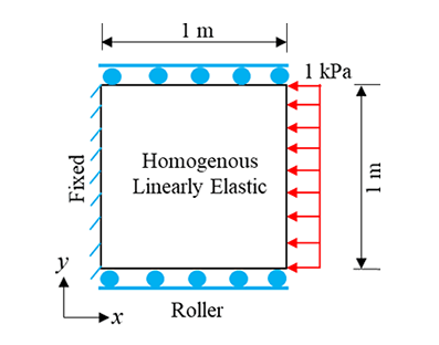
A distributed load of 1 kPa is applied on the right side of a square element. As shown in the following figure, the element has a side length of 1 m. The material consisting the element has a Young's modulus of 10 GPa and a Poisson's ratio of 0.2. The left boundary is fixed while the upper and lower boundary was constrained using "rollers": displacement is allowed along the boundary surface while not allowed along the normal direction. A plane strain condition is assumed for this 2D problem. Please calculate the stress distribution inside of the element.