Fluid Dynamics
Introduction
Fluid dynamics, as a study area, has a much broader scope than the fluid dynamics discussed in the context of multiphysics. The solution to a fluid dynamics problem typically involves the calculation of the spatial (and temporal) variations of various properties of a fluid, such as flow velocity, pressure, density, and temperature. These calculations are built on the conservation of mass, momentum, and energy, especially the first two. These axioms of conservation lead to the mathematical formulation of the fluid flow: Navier-Stokes equations.
$\space$Compressible Newtonian fluid
Directly substituting the above constitutive relationship into the general N-S equations yields the N-S equations for the flow of compressible Newtonian fluids:
\[\rho \left(\frac{\partial v}{\partial t} +v\cdot \nabla v\right)=-\nabla p+\nabla \cdot \left\{\mu \left[\nabla v+\left(\nabla v\right)^{T} \right]\right\}+\nabla \left(-\frac{2\mu }{3} \nabla \cdot v\right)+\rho g, \]where $p$ is used to represent the pressure, and the gravity is considered as the only body force, i.e.$f=\rho g$. The associated mass continuity equation is
\[\frac{\partial \rho }{\partial t} +\nabla \cdot \left(\rho v\right)=0. \]The above form of the N-S equations can cover the dynamics of most gases and liquids with a good equation of state and good functions for the dependence of parameters such as viscosity on the variables.
$\space$Incompressible Newtonian Fluid
The N-S equations for incompressible Newtonian fluids can be derived from the equations for compressible fluids with two further simplifications.
The viscosity $\mu $ is a constant.
The second viscosity coefficient diminishes, $\lambda =0$.
As the fluid is incompressible, the mass balance equation is simply transformed into
\[\nabla \cdot v=0.\]The N-S equations for incompressible Newtonian fluids are
\[\nabla \cdot u=0\] \[\rho \left(\frac{\partial u}{\partial t} +u\cdot \nabla u\right)=-\nabla p+\mu \nabla ^{2} u+\rho g. \]It is also common to write the momentum equation in the following form
\[\frac{\partial u}{\partial t} +u\cdot \nabla u=-\nabla e+\nu \nabla ^{2} u+g, \]where $e$ is the specific (per unit mass) thermodynamic work and $ \nu=\mu / \rho$ is the kinematic viscosity.
$\space$Turbulent Models
As mentioned above, the discrete nature of the fluid flow can significantly deviate the flow condition from what would be predicted using the N-S equations discretized at large scales. This is because the randomness and chaos caused by the discrete nature can change the flow patterns via couplings between different scales. The resultant recirculation, eddies, and apparent randomness are characterized as turbulence. The key idea to separate turbulence from the mean flow is averaging. The Reynolds averaging technique operates as follows,
\[\phi \left(x,t\right)=\bar{\phi }\left(x,t\right)+\phi ^{'} \left(x,t\right),\]where $\phi \left(x,t\right)$ is decomposed into an average term $\bar{\phi }\left(x,t\right)$ and an oscillating term $\phi ^{'} \left(x,t\right)$. $\phi ^{'} \left(x,t\right)$ denotes the fluctuation around the mean value, which is defined as
\[\bar{\phi }\left(x,t\right)={\mathop{\lim }\limits_{N\to \infty }} \frac{1}{N} \mathop{\sum }\limits_{i=1}^{N} \phi _{i} \left(x,t\right), \]where N is the number of identically performed experiments.
Applying the above averaging procedure to the incompressible N-S equations, the following form of the averaged equations can be obtained:
\[\nabla \cdot \bar{v}=0, \] \[\frac{\partial \bar{v}}{\partial t} +\nabla \cdot \left(\bar{v}\bar{v}\right)=g-\nabla \bar{p}+\nabla \cdot \left(\nu \nabla \bar{v}+{\mathop{v^{'} v^{'} }\limits^{\_ \_ \_ \_ \_ }} \right), \]where the term ${\mathop{v^{'} v^{'} }\limits^{\_ \_ \_ \_ \_ }} $ is called the Reynolds stress tensor. In order to close the system, further modeling is necessary to obtain the Reynolds stress.
The most popular approach is to use the Boussinesq approximation (Boussinesq eddy viscosity hypothesis) [Schmitt, 2007], which adopts a linear relation of the form:
\[{\mathop{v^{'} v^{'} }\limits^{\_ \_ \_ \_ \_ }} =-v_{t} \left[\nabla \bar{v}+\left(\nabla \bar{v}\right)^{T} \right]+\frac{2}{3} kI, \] where $k=\frac{1}{2} {\mathop{v^{'} }\limits^{\_ \_ }} \cdot {\mathop{v^{'} }\limits^{\_ \_ }} $.The kinematic eddy viscosity $v_{t} $ can be evaluated in many different ways, ranging from algebraic relations and local equilibrium assumptions to the solution of transport equations. The most popular approach is to express $v_{t} $ as a function of the turbulent kinetic energy k and its dissipation rate $\varepsilon $, leading to a "two-equation" turbulence model:
\[v_{t} =C_{\mu } \frac{k^{2} }{\varepsilon } , \] \[\varepsilon =v{\mathop{v^{'} v^{'} :\nabla v^{'} }\limits^{\_ \_ \_ \_ \_ \_ \_ \_ \_ \_ \_ \_ \_ }} .\]In this type of turbulent model, $k$ and $\varepsilon $ are obtained by the solution of their respective transport equations. The first model of this kind was proposed by Harlow and Nakayama [1968]. Derivation of the transport equations for $k$ and $\varepsilon $ can be found in Launder and Spalding [1974]. In fact, a wide variety of $k$-$\varepsilon $ models exist, while the most noteworthy one is the standard $k$-$\varepsilon $ model proposed by Launder and Spalding [1974] and the RNG $k$-$\varepsilon $ variant proposed by Yakhot and Orszag [1986] and Yakhot et al. [1992].
The exact $k$-$\varepsilon $ equations contain many unknown and unmeasurable terms. For a much more practical approach, the standard $k$-$\varepsilon $ turbulence model [Launder and Spalding,1974] is used. This model was established based on our best understanding of the relevant processes and thus minimizes the number of unknowns and leads to a set of equations which can be applied to a large number of turbulent applications.
For turbulent kinetic energy $k$, we have
\[\frac{\partial \left(\rho k\right)}{\partial t} +\frac{\partial \left(\rho kv_{i} \right)}{\partial x_{i} } =\frac{\partial }{\partial x_{j} } \left(\frac{\mu _{t} }{\sigma _{k} } \frac{\partial k}{\partial x_{j} } \right)+2\mu _{t} E_{ij} E_{ij} -\rho \varepsilon . \]For dissipation $\varepsilon $, a similar transport equation can be used,
\[\frac{\partial \left(\rho \varepsilon \right)}{\partial t} +\frac{\partial \left(\rho \varepsilon v_{i} \right)}{\partial x_{i} } =\frac{\partial }{\partial x_{j} } \left(\frac{\mu _{t} }{\sigma _{\varepsilon } } \frac{\partial \varepsilon }{\partial x_{j} } \right)+C_{1\varepsilon } \frac{\varepsilon }{k} 2\mu _{t} E_{ij} E_{ij} -C_{2\varepsilon } \rho \frac{\varepsilon ^{2} }{k} ,\]where $v_{i} $ is the velocity component in the corresponding direction; $E_{ij} $ is the component of the rate of deformation; and $\mu _{t} $ is the eddy viscosity, which can be calculated as $\mu _{t} =\rho C_{\mu } \frac{k^{2} }{\varepsilon } $.
The above equation states the following balance:
Rate of change of $k$ or $\varepsilon $+ Transport of $k$ or $\varepsilon $ by convection= Transport of $k$ (or $\varepsilon $) by diffusion+ Rate of production of $k$ (or $\varepsilon $) - Rate of the destruction of $k$ (or $\varepsilon $).
The equations also consist of some adjustable constants: $\sigma _{k} $, $\sigma _{\varepsilon } $, $C_{1\varepsilon } $ and$C_{2\varepsilon } $. The values of these constants have been obtained by numerous iterations of data fitting for a wide range of turbulent flows. A common set of values are as follows: $C_{\mu } $=0.09, $\sigma _{k} $=1.00, $\sigma _{\varepsilon } $=1.30, $C_{1\varepsilon } $=1.44, and $C_{2\varepsilon } $=1.92.
$\space$Example
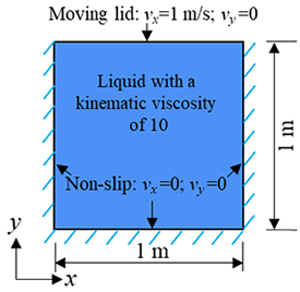
In a 1 m by 1 m square liquid container as shown in the following figure, the liquid inside the container moves as the lid on the top boundary continuously moves from the left to the right at a velocity of 1 m/s. Assuming the water on the top boundary moves at the same speed as the lid, please predict the distribution of $v_{x} $ along $x$= 0.5 m and $v_{y} $ along $y$= 0.5 m and compare them against the numerical results of Ghia et al. [1982]. The kinematic viscosity is 10.

Results
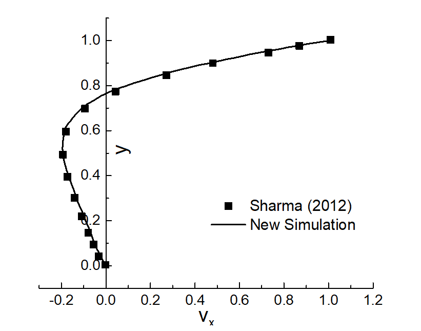
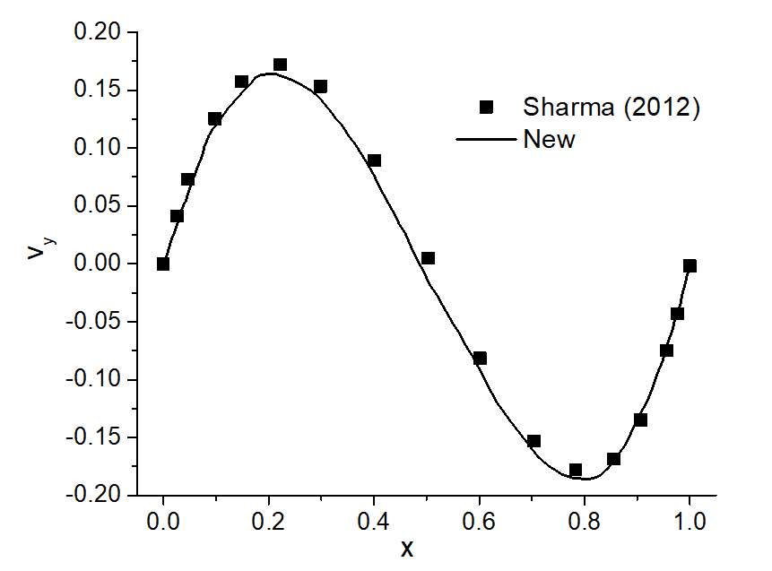
The results obtained by the numerical simulation implemented with FlexPDE are compared against the results given in Sharma [2012]. As shown in the following two figures, a simple CFD implementation with a very coarse mesh and the finite element method can also generate acceptable results. Better comparisons can be obtained by further tuning the numerical model and solution techniques.


